
Summary
It has been asked why the charts of maximum Type I error in the paper have a sawtooth appearance (for example, as in Figure 1 of the main paper reproduced below). This page provides the explanation.
Figure 1 of Statistics in Medicine paper
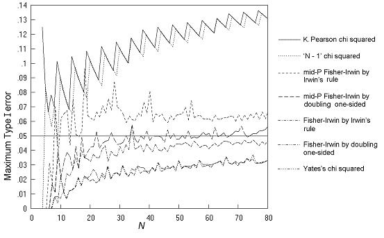
This sawtooth appearance is particularly evident for comparative trials analysed by the K Pearson chi squared and 'N - 1' chi squared tests (Figure 1 of the main paper, reproduced above). In summary, it can be described as due to the arbitrary nature of the 5% or other cutoff. The following tables and charts for comparative trials analysed by the K Pearson chi squared test give some detail to this.
Table A shows the data for first two teeth that appear in the solid line on Figure 1 of the main paper. As N increases, the maximum Type I error falls steadily from 0.1015 for N = 9 to 0.0683 at N = 13, and then jumps up to 0.1047 at N = 14. Then there is again a steady decline followed by a further jump at N = 19. The values of π (the population proportion in column 1) and m (the number in row 1) that give these maxima are also shown in Table A. This shows that the maximum Type I error occurs at fairly extreme values of π and very extreme values of m, as has been found in previous studies (this point will be returned to below).
Table A: Comparative trials analysed by the K Pearson chi squared test (alpha = 5%): the maximum Type I error over all values of π and all possible m, n pairs with an inaccuracy of less than 0.001
| ----------------------------------------------------------------------------------------------------------- | |||
| N | Max Type I error | π at Max Type I error | m at Max Type I error |
| ----------------------------------------------------------------------------------------------------------- | |||
| 9 | 0.1015 | 0.182 | 1 |
| 10 | 0.0905 | 0.164 | 1 |
| 11 | 0.0816 | 0.148 | 1 |
| 12 | 0.0744 | 0.135 | 1 |
| 13 | 0.0683 | 0.125 | 1 |
| 14 | 0.1047 | 0.165 | 1 |
| 15 | 0.0972 | 0.155 | 1 |
| 16 | 0.0908 | 0.145 | 1 |
| 17 | 0.0851 | 0.135 | 1 |
| 18 | 0.0802 | 0.128 | 1 |
| 19 | 0.1084 | 0.158 | 1 |
| 20 | 0.1026 | 0.150 | 1 |
| ----------------------------------------------------------------------------------------------------------- | |||
Table B gives more detail by showing the sample tables that are significant at 5% at the maximum Type I error. From N = 9 to N = 13, there are just four significant sample tables and the pattern of tables is the same in each case, namely (1 0 0 N-1), (1 0 1 N-2) and two similar tables by symmetry; with the frequency gradually falling (as N increases and there are a larger number of sample tables). When N reaches 14, the number of significant tables increases from 2 pairs to 3 pairs, and this is the reason for the jump in the total Type I error; it is because of the addition of the extra pair of sample tables of the form (1 0 2 N-3). Similarly, the jump in total Type I error when N reaches 19 is because of the addition of a further pair of tables of the form (1 0 3 N-4). So the saw-tooth pattern in this case is just a result of the arbitrary nature of the cutoff of 5%. Other situations studied were similar - the large steps up in total Type I error as N increases are due to the inclusion of an additional class of table in the set of significant tables, which at smaller N was not quite significant.
Table B: Comparative trials analysed by the K Pearson chi squared test : List of sample tables that are significant at 5% with the frequency of each table at the values of π and m that give the maximum Type I error
| ----------------------------------------------------------------------------------------------------------- | |||||||
| N | Max Type | @π | @m | Table | P value | Frequency | Cumulative |
| I error | a b c d | frequency | |||||
| ----------------------------------------------------------------------------------------------------------- | |||||||
| 9 | .1015 | .182 | 1 | ||||
| 1 0 0 8 | 0.0027 | 3.65E-02 | |||||
| 0 1 8 0 | 0.0027 | 9.85E-07 | 0.0365 | ||||
| 1 0 1 7 | 0.047 | 6.49E-02 | |||||
| 0 1 7 1 | 0.047 | 3.54E-05 | 0.1015 | ||||
| 10 | .0905 | .164 | 1 | ||||
| 1 0 0 9 | 0.0016 | 3.27E-02 | |||||
| 0 1 9 0 | 0.0016 | 7.17E-08 | 0.0327 | ||||
| 1 0 1 8 | 0.035 | 5.78E-02 | |||||
| 0 1 8 1 | 0.035 | 3.29E-06 | 0.0905 | ||||
| 11 | .0816 | .148 | 1 | ||||
| 1 0 0 10 | 0.0009 | 2.98E-02 | |||||
| 0 1 10 0 | 0.0009 | 4.30E-09 | 0.0298 | ||||
| 1 0 1 9 | 0.026 | 5.18E-02 | |||||
| 0 1 9 1 | 0.026 | 2.47E-07 | 0.0816 | ||||
| 12 | .0744 | .135 | 1 | ||||
| 1 0 0 11 | 0.0005 | 2.74E-02 | |||||
| 0 1 11 0 | 0.0005 | 2.35E-10 | 0.0274 | ||||
| 1 0 1 10 | 0.020 | 4.70E-02 | |||||
| 0 1 10 1 | 0.020 | 1.65E-08 | 0.0744 | ||||
| 13 | .0683 | .125 | 1 | ||||
| 1 0 0 12 | 0.0003 | 2.52E-02 | |||||
| 0 1 12 0 | 0.0003 | 1.27E-11 | 0.0252 | ||||
| 1 0 1 11 | 0.015 | 4.32E-02 | |||||
| 0 1 11 1 | 0.015 | 1.07E-09 | 0.0683 | ||||
| 14 | .1047 | .165 | 1 | ||||
| 1 0 0 13 | 0.0002 | 1.58E-02 | |||||
| 0 1 13 0 | 0.0002 | 5.61E-11 | 0.0158 | ||||
| 1 0 1 12 | 0.011 | 4.07E-02 | |||||
| 0 1 12 1 | 0.011 | 3.69E-09 | 0.0565 | ||||
| 1 0 2 11 | 0.047 | 4.82E-02 | |||||
| 0 1 11 2 | 0.047 | 1.12E-07 | 0.1047 | ||||
| 15 | .0972 | .155 | 1 | ||||
| 1 0 0 14 | 0.0001 | 1.47E-02 | |||||
| 0 1 14 0 | 0.0001 | 3.90E-12 | 0.0147 | ||||
| 1 0 1 13 | 0.0083 | 3.77E-02 | |||||
| 0 1 13 1 | 0.0083 | 2.98E-10 | 0.0523 | ||||
| 1 0 2 12 | 0.038 | 4.49E-02 | |||||
| 0 1 12 2 | 0.038 | 1.06E-08 | 0.0972 | ||||
| 19 | .1084 | .158 | 1 | ||||
| 1 0 0 18 | 1.307E-05 | 7.15E-03 | |||||
| 0 1 18 0 | 1.307E-05 | 3.17E-15 | 0.0071 | ||||
| 1 0 1 17 | 0.0027 | 2.41E-02 | |||||
| 0 1 17 1 | 0.0027 | 3.04E-13 | 0.0313 | ||||
| 1 0 2 16 | 0.018 | 3.85E-02 | |||||
| 0 1 16 2 | 0.018 | 1.38E-11 | 0.0698 | ||||
| 1 0 3 15 | 0.047 | 3.85E-02 | |||||
| 0 1 15 3 | 0.047 | 3.92E-10 | 0.1084 | ||||
| ----------------------------------------------------------------------------------------------------------- | |||||||
This step change at particular values of N in Type I error at a specified significance level means that assessing tests in this way is not entirely satisfactory, but it is the simplest method, and also the most used in previous studies, and so it was the main method chosen to present the results of this work.
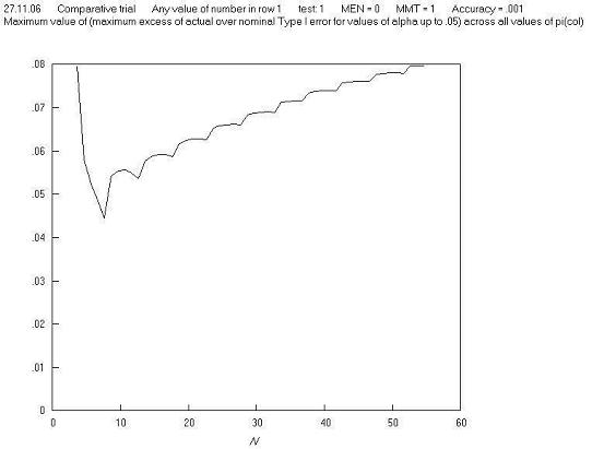
There is a more complex method developed as part of this work. This is to assess the maximum Type I error excess, which can be explained by reference to Table B. Looking at the four sample tables when N = 9, the total Type I error is 0.1015. Even if the total had been 0.05, the test would not be acting as an ideal test, because the P values of the four tables are only up to 0.047 - an ideal test would have a cumulative frequency of tables that was equal to the largest P value, i.e. equal to 0.047. Similarly, at N = 10, since the largest P value of the four tables is 0.035, the cumulative frequency of tables up to and including this should be 0.035, but instead is 0.0905, i.e. too large by 0.056. This value of 0.056 can be termed the excess Type I error, and this in fact changes very little with N. Figure A plots the maximum Type I error excess against N, rather than the maximum Type I error, and it can be seen that the sawtooth effect has largely disappeared.
Figure A
Type I error and row 1 marginal total
Returning to the point that the maximum Type I error in the above example occurs when m = 1: this means that when m = 1, a chart of the maximum Type I error across all values of π for Pearsons chi squared test mostly repeats the solid line of Figure 1 of the paper. This is shown in Figure B.
Figure B
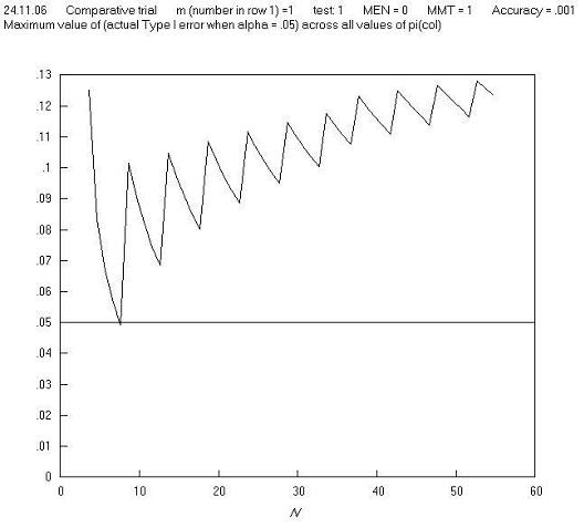
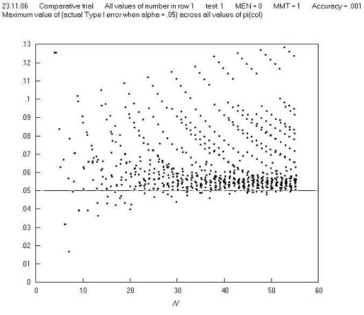
A first reaction to this finding is that in real life, comparative trials are not carried out (or should not be carried out) where one group has just one observation. So perhaps we need to set a criterion that 2 x 2 tables should not be analysed if a marginal total is equal to just 1, and this might remove the high Type I errors; but further charts show that this is not the case: Figures C and D show a repeat of Figure B, but with m = 2 and m = 3 respectively, and Figure E shows the maximum Type I error across all values of π for all m, n pairs. These and other charts show that limitation in terms of a minimum marginal total is not effective in avoiding high Type I errors. Further charts of Type I error against π for different values of m and N show that the high Type I errors occur just at extremes of both π and m, and so in order to make the Pearson (and 'N - 1') chi squared test perform well, we need to avoid using them in situations where there both π and m are extreme. Fortunately, the restriction in terms of minimum expected cell number achieves this, as it is equal to the product of π (estimated from the sample) and m (when cell a is the smallest cell, as is the convention here).
Figure C
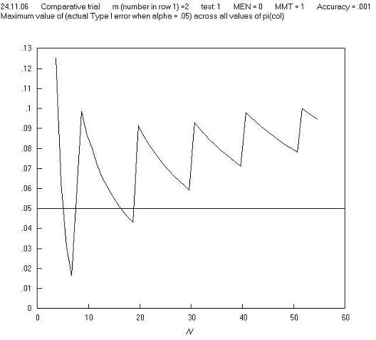
Figure D
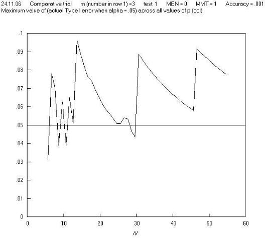
Figure E
Back to top