
Summary
This page expands on the methods section published in the paper: Campbell Ian, 2007, Chi-squared and Fisher-Irwin tests of two-by-two tables with small sample recommendations, Statistics in Medicine, 26, 3661 - 3675.
The research compared methods of analysis of 2 x 2 tables, focusing on seven two-sided tests: three versions of the chi squared test and four versions of the Fisher-Irwin test:
(1) K. Pearson's chi squared test, comparing (ad - bc)2N / mnrs with the chi squared distribution with one degree of freedom;
(2) Yates's chi squared test, comparing (|ad - bc| - ½N)2N / mnrs with the chi squared distribution (Yates, 1934). Although not specified by Yates in his paper, it is usual not to take the adjustment by ½N beyond zero, and this convention was adopted here.
(3) 'N - 1' chi squared test, comparing (ad - bc)2(N - 1) / mnrs with the chi squared distribution.
(4) The Fisher-Irwin test, by doubling the one-sided P value. For tables that are close to statistical significance, the procedure is generally clear-cut, but for tables that are far from significance, some clarification is needed. In obtaining the one-sided value, Fisher (1935) described adding the probabilities of tables with the same marginal totals that have 'a discrepancy from proportionality as great or greater than that observed'. Many textbooks give the procedure as progressively decrementing the smallest cell of the table, but this can give misleading P values, for example from the table (2 3 4 21); and it is better to take the tail of the distribution of possible tables with the smaller total probability (Jagger, 1984; Yates, 1984, p461). If both directions give totals greater than 0.5, the table can be regarded as a central table, not belonging to either tail, with a two-sided probability of 1 (Yates, 1984). These procedures (i.e. those recommended by Yates) were used for this version of the Fisher-Irwin test in this study.
(5) The Fisher-Irwin test, taking tables from either tail as likely, or less, as that observed (Irwin's rule);
(6) The mid-P Fisher-Irwin test, by doubling the one-sided mid-P level;
(7) The mid-P Fisher-Irwin test, using Irwin's rule.
Comparison of P values with ideal behaviour
Calculations were carried out using software written in Microsoft Visual Basic version 6. The program is available from this website.
The user interface (see above) allows the research design to be specified as either a comparative trial or a cross-sectional study; and allows specification of the sample size(s) and null hypothesis population proportion(s). The set of all possible samples with their probability is generated via the relevant standard probability formula (Barnard, 1947a); for example the probability formula for the table (a b c d) in a comparative trial is given by expression (1) (see background information). The P values by the seven tests are calculated by purpose-written routines. Chi squared values are converted to P values via calculation of the normal integral, using an algorithm with an inaccuracy in the P value of less than 0.0001. The program saves the possible sample tables with their probabilities and P values to a disk file (to allow verification and detailed investigation), and displays the P values as cumulative frequency charts. As well as allowing the setting of particular values of sample sizes and population parameters, the software allows a sequence of values to be specified such as a total sample size of '10 to 50 step 2'. The program displays summary charts such as Type I error at particular α and π against total sample size.
Calculation of maximum Type I errors in a comparative trial over all values of π
For specified sample sizes and α, the maximum Type I error across all values of π cannot be determined analytically, but it can be obtained by the following numerical method to an acceptable degree of accuracy. For a comparative trial, the value to be determined is the maximum value of the sum of the probabilities of those tables that are significant at the chosen α. These probabilities are given by expression (1) (see background information), and so the total is a sum of polynomials in π and is therefore a smooth but possibly multimodal function of π. Except for tables with zero marginal totals (see above), the probability (1) of any particular table increases from a value of zero at π = 0, to a maximum value at π = r/N, and then decreases again to zero at π = 1. So for any interval in π from πL to πU, the maximum value of the probability over the interval will be at πL if r/N ≤ πL, at πU if r/N ≥ πU, and otherwise will be at r/N. By summing the interval maximum values of the probabilities of the significant tables, we can obtain an upper bound to the maximum value of the Type I error over that interval. This upper bound will in general be larger than the actual maximum because the maximum probabilities for the significant tables will generally occur at different values of π. However, the narrower the interval, the smaller will be the difference between the upper bound and actual maximum, and by making the interval sufficiently narrow, the difference (and therefore the inaccuracy in the estimate) can be made as small as we like. So if we divide the range of possible values of π into a number of intervals, we can calculate an upper bound of the Type I error for each interval, and the largest of these upper bounds across all the intervals is an upper bound to the overall maximum Type I error. Values of π can lie between 0 and 1, but for a two-sided test, there is symmetry around 0.5 and we need consider π only the range 0 to 0.5.
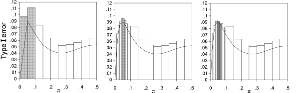
Fig. 3. Illustration of the algorithm used to determine the maximum Type I error across all values of π in comparative trials. The example shown is for N = 30, m = 24, n = 6, with analysis by Pearson's chi squared test at a nominal value of 0.05, and inaccuracy of less than 0.002.
The details of the algorithm used are as follows, and are illustrated in Fig. 3, which shows charts generated by the program, when determining the maximum Type I error by the Pearson chi squared test at a nominal value of 5%, for a comparative trial with group sizes of 24 and 6. The accuracy δ was specified as 0.002. On the first iteration, the range of values of π of 0 to 0.5 was divided into ten equal intervals. Point values of the Type I error were calculated at the 11 boundaries of the intervals, and are shown in Fig. 3(a) by the solid line joining them. The upper bounds calculated for the Type I errors are shown by the rectangles for each interval. The largest point value was 0.0901 at π = 0.05. For eight of the intervals (shown by white rectangles), the interval upper bound was less than 0.0901 + δ i.e. was less than 0.0921, and so these intervals cannot contain a Type I error greater than the largest point value found (to an accuracy of δ). These intervals were consequently discarded from further investigation. The remaining two intervals (shown by the grey rectangles) had Type I error upper bounds greater than 0.0921, and so were retained for further analysis. A second iteration divided this restricted range into narrower intervals of equal size (Fig. 3b) and the process was repeated. With these narrower intervals, the upper bounds were smaller, and closer to the point values. The number of intervals is kept the same at each iteration provided the range of values of π is narrowed to one half or less at the previous iteration - otherwise it is doubled. The iterations continued until all the interval upper bounds were smaller than the highest point value plus δ, giving in this example, a maximum of 0.0905 at π = 0.046 (Fig. 3c). The accuracies specified were generally less than 1/20 of the nominal Type I error. This method has some similarities to that of Suissa and Shuster (1985), although developed independently.
Calculation of maximum Type I errors in a cross-sectional study over all values of π1 and π2
For a cross-sectional study, in order to find the maximum Type I error, we need to find the maximum over every possible pair of values of π1 and π2, except that, with symmetry for a two-sided test around 0.5, we need consider only values of π1 and π2 between 0 and 0.5; and furthermore, without loss of generality, we can consider only combinations where π1 ≥ π2. In this study, the maximum Type I error for cross-sectional studies was determined by an extension of the method for comparative trials described above. Instead of considering one-dimensional intervals in π, the method involves study of two-dimensional areas of the combined space of π1 and π2.
In outline, the process starts with the entire two-dimensional space, and progressively focusses on that part of it that contains the maximum value. This is done by progressively eliminating strips of the space where the upper bound can be shown to be less than the largest point value found, to an accuracy δ. The process is illustrated in Fig. 4, which is a set of figures generated by the program. The initial two-dimensional space, represented by the upper triangle, was divided by a grid, and the point values at the intersections of the grid lines were calculated, and so were upper bounds for the Type I error for each rectangular area marked out by the grid lines. These upper bounds were calculated in the same way as for comparative trials, except that the probability for each table now depends on the product of terms in π1 and terms in π2, and so the upper bound of the Type I error was obtained from summing for each significant table the product of the maximum value in the area of the terms in π1 and the maximum value of the terms in π2. The highest point value was obtained across all grid intersections. If the upper bound in any area was less than the overall maximum point value + δ, then that area could be marked as not containing the overall maximum value, to an accuracy of δ. Where an entire row or an entire column of areas is so recorded, then that strip could be excluded from the region in the combined space of π1 and π2 that contains the maximum Type I error to an accuracy of δ. The process was repeated iteratively, considering progressively smaller sized areas, and removing strips of areas that did not contain the overall maximum to an accuracy of δ, until the upper bounds of all the areas in the residual region were less than the largest point value + δ.
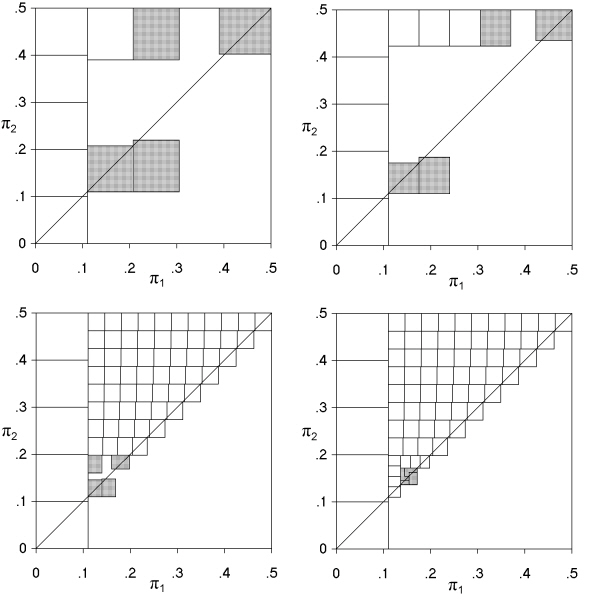
Fig. 4. Illustration of the algorithm used to determine the maximum Type I error across all values of π1 and π2. The example shown is the first (a), second (b), fourth (c) and sixth (d) iterations in a cross-sectional study of size N = 10, with analysis by Pearson's chi squared test at a nominal value of 0.05, and inaccuracy of less than 0.005.
Fig. 4 illustrates the method in detail for the case of the determination of the maximum Type I error to an accuracy (δ) of 0.005 in a cross-sectional study of sample size 10, when analysed by the Pearson chi squared test with a nominal α of 0.05. In the first iteration, an initial survey of a six-by-six grid gave the largest Type I error to be 0.0577 at a position (π1, π2) of (0.167, 0.167); and investigation of individual areas (Fig. 4a) showed that the upper bounds for six of them (shown white) were less than 0.0577 + δ, i.e. less than 0.0627. Five of these areas constituted the left hand strip, and the corresponding values of π1 could be marked as not containing the maximum Type I error. In other areas (marked grey) the upper bounds were above 0.0627. All areas except the left hand strip were retained for further examination. In the subsequent iterations, investigation of progressively smaller areas gave no complete strips that could be excluded until the fourth iteration. After this, a survey of the residual space gave the largest Type I error to be 0.0580 at a position (0.154, 0.154), with a largest upper bound of 0.0632. After the sixth iteration, the residual space that contained the largest Type I area to accuracy δ was narrowed further, and a survey of this space again gave the largest Type I error to be 0.0580 at (0.154, 0.154), with a largest upper bound of 0.0602, which was less than 0.0630, and so the calculation had been finalised.
In fact, the largest calculated Type I error changes little when the specified accuracy is increased, changing from 0.057990 at a specified accuracy of 0.005, to 0.05799406 at 0.0005, and 0.05799407 at 0.00005. This indicates that the actual accuracy obtained by the algorithm is many times greater than the specified accuracy, and this was a general finding in both cross-sectional and comparative research designs.
Similar methods were used for comparative trials and cross-sectional studies to determine the maximum value over all population proportion(s) of the Type I error excess over a range of nominal values up to 5% (or other specified value). On P value cumulative frequency charts, this is the largest distance over all values of π of the cumulative frequency above the diagonal for P values up to 5% (or other value). Another end-point considered was the opposite quantity: the largest distance below the diagonal on the P value cumulative frequency chart over all population proportion(s), but this is not an informative quantity as the cumulative frequency chart tends to the x axis at low population proportion(s).
The program speed was enhanced by minimising computations e.g. by storing in computer memory the values of factorials, of P values for particular tables, and of the P value orderings for particular sample sizes, so that these were calculated no more than necessary. The program was verified by checks of internal consistency, by the writing of intermediate stages in the calculations to disk files to facilitate checking, and by the replication of 29 example P values, tables or charts from 14 previous publications: Barnard (1989), Berkson (1978a), Bradley and Cutcomb (1977), Garside and Mack (1976), Haber (1986), Hwang and Yang (2001), Irwin (1935), Kurtz (1968), Pearson (1947), Rice (1988), Richardson (1990), Schouten et al. (1980), Storer and Kim (1990), and Upton (1982). Some of these replications of previously published results are included as example settings within the program.
Power and ordering of the sample space
Tests were compared in pairs in the analysis of cross-sectional studies of sizes equal to all integers from 4 to 80, to determine the extent to which the rejection region at P < 5% for one test is a subset of that for the other test.
Back to top